Generating a single cell matrix using Alevin
Overview
Questions:Objectives:
I have some single cell FASTQ files I want to analyse. Where do I start?
Requirements:
Repeat matrix generation for any droplet-based single cell sequencing data
Apply data combination and metadata editing for particular experimental designs
Interpret quality control (QC) plots to make informed decisions on cell thresholds
Find relevant information in GTF files for the particulars of their study, and include this in data matrix metadata
- Introduction to Galaxy Analyses
- Sequence analysis
- Quality Control: slides slides - tutorial hands-on
- Mapping: slides slides - tutorial hands-on
- Transcriptomics
- An introduction to scRNA-seq data analysis: slides slides
- Understanding Barcodes: tutorial hands-on
Time estimation: 3 hoursSupporting Materials:
- Topic Overview slides
- Datasets
- Workflows
- FAQs
- video Recordings
- instances Available on these Galaxies
Last modification: Mar 1, 2022
Introduction
This tutorial will take you from raw FASTQ files to a cell x gene data matrix in AnnData format. What’s a data matrix, and what’s AnnData format? Well you’ll find out! Importantly, this is the first step in processing single cell data in order to start analysing it. Currently you have a bunch of strings of ATGGGCTT etc. in your sequencing files, and what you need to know is how many cells you have and what genes appear in those cells. In the second part of this tutorial, we will also look at combining FASTQ files and adding in metadata (for instance, SEX or GENOTYPE) for analysis later on. These steps are the most computationally heavy in the single cell world, as you’re starting with 100s of millions of reads, each 4 lines of text. Later on in analysis this data becomes simple gene counts such as ‘Cell A has 4 GAPDHs’, which is a lot easier to store! Because of this data overload, we have downsampled the FASTQ files to speed up the analysis a bit. Saying that, you’re still having to map loads of reads to the massive murine genome, so get yourself a cup of coffee and prepare to analyse!
Agenda
In this tutorial, we will cover:
Generating a matrix
In this section, we will show you the principles of the initial phase of single-cell RNA-seq analysis: generating expression measures in a matrix. We’ll concentrate on droplet-based (rather than plate-based) methodology, since this is the process with most differences with respect to conventional approaches developed for bulk RNA-seq.
Droplet-based data consists of three components: cell barcodes, unique molecular identifiers (UMIs) and cDNA reads. To generate cell-wise quantifications we need to:
- Process cell barcodes, working out which ones correspond to ‘real’ cells, which to sequencing artefacts, and possibly correct any barcodes likely to be the product of sequencing errors by comparison to more frequent sequences.
- Map biological sequences to the reference genome or transcriptome.
- ‘De-duplicate’ using the UMIs.
This used to be a complex process involving multiple algorithms, or was performed with technology-specific methods (such as 10X’s ‘Cellranger’ tool) but is now much simpler thanks to the advent of a few new methods. When selecting methodology for your own work you should consider:
- STARsolo - a droplet-based scRNA-seq-specific variant of the popular genome alignment method STAR. Produces results very close to those of Cellranger (which itself uses STAR under the hood).
- Kallisto/ bustools - developed by the originators of the transcriptome quantification method, Kallisto.
- Alevin - another transcriptome analysis method developed by the authors of the Salmon tool.
We’re going to use Alevin Srivastava et al. 2019 for demonstration purposes, but we do not endorse one method over another.
Get Data
We’ve provided you with some example data to play with, a small subset of the reads in a mouse dataset of fetal growth restriction Bacon et al. 2018 (see the study in Single Cell Expression Atlas here and the project submission here). This is a study using the Drop-seq chemistry, however this tutorial is almost identical to a 10x chemistry. We will point out the one tool parameter change you will need to run 10x samples. This data is not carefully curated, standard tutorial data - it’s real, it’s messy, it desperately needs filtering, it has background RNA running around, and most of all it will give you a chance to practice your analysis as if this data were yours.
Down-sampled reads and some associated annotation can be downloaded from Zenodo below, or you can import this example input history. How did I downsample these FASTQ files? Check out this history to find out! Additionally, to map your reads, you will need a transcriptome to align against (a FASTA) as well as the gene information for each transcript (a gtf) file. You can download these for your species of interest from Ensembl here. Additionally, these files are available in the above history as well as the Zenodo links below. Keep in mind, these are big files, so they may take a bit to import!
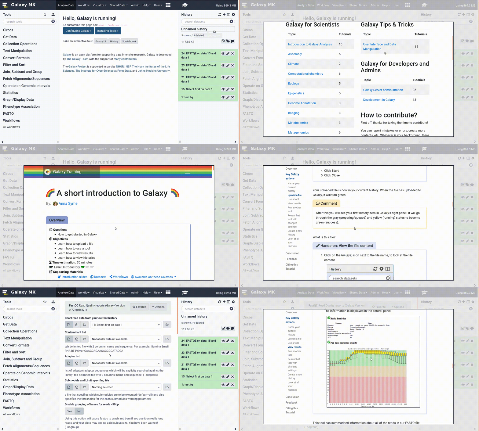
hands_on Hands-on: Data upload - Part 1
- Create a new history for this tutorial
Import the Experimental Design table, sequencing reads 1 & 2, the GTF and fasta files from Zenodo
https://zenodo.org/record/4574153/files/Experimental_Design.tabular
https://zenodo.org/record/4574153/files/Mus_musculus.GRCm38.100.gtf.gff
https://zenodo.org/record/4574153/files/Mus_musculus.GRCm38.cdna.all.fa.fasta
https://zenodo.org/record/4574153/files/SLX-7632.TAAGGCGA.N701.s_1.r_1.fq-400k.fastq
https://zenodo.org/record/4574153/files/SLX-7632.TAAGGCGA.N701.s_1.r_2.fq-400k.fastq
Tip: Importing via links
- Copy the link location
Open the Galaxy Upload Manager (galaxy-upload on the top-right of the tool panel)
- Select Paste/Fetch Data
Paste the link into the text field
Press Start
- Close the window
- Rename galaxy-pencil the datasets
question Questions
Have a look at the files you now have in your history.
- Which of the FASTQ files do you think contains the barcode sequences?
- Given the chemistry this study should have, are the barcode/UMI reads the correct length?
- What is the ‘N701’ referring to?
solution Solution
- Read 1 (SLX-7632.TAAGGCGA.N701.s_1.r_1.fq-400k) contains the cell barcode and UMI because it is significantly shorter (indeed, 20 bp!) compared to the longer, r_2 transcript read. For ease, rename these files N701-Read1 and N701-Read2.
- You can see Read 1 is only 20 bp long, which for original Drop-Seq is 12 bp for cell barcode and 8 bp for UMI. This is correct! Be warned - 10x Chromium (and many technologies) change their chemistry over time, so particularly when you are accessing public data, you want to check and make sure you have your numbers correct!
- ‘N701’ is referring to an index read. This sample was run alongside 6 other samples, each denoted by an Illumina Nextera Index (N70X). Later, this will tell you batch information. If you look at the ‘Experimental Design’ file, you’ll see that the N701 sample was from a male wildtype neonatal thymus.
Generate a transcript to gene map
Gene-level, rather than transcript-level, quantification is standard in scRNA-seq, which means that the expression level of alternatively spliced RNA molecules are combined to create gene-level values. Droplet-based scRNA-seq techniques only sample one end each transcript, so lack the full-molecule coverage that would be required to accurately quantify different transcript isoforms.
To generate gene-level quantifications based on transcriptome quantification, Alevin and similar tools require a conversion between transcript and gene identifiers. We can derive a transcript-gene conversion from the gene annotations available in genome resources such as Ensembl. The transcripts in such a list need to match the ones we will use later to build a binary transcriptome index. If you were using spike-ins, you’d need to add these to the transcriptome and the transcript-gene mapping.
In your example data you will see the murine reference annotation as retrieved from Ensembl in GTF format. This annotation contains gene, exon, transcript and all sorts of other information on the sequences. We will use these to generate the transcript/ gene mapping by passing that information to a tool that extracts just the transcript identifiers we need.
question Questions
Which of the ‘attributes’ in the last column of the GTF files contains the transcript and gene identifiers?
tip Hint
The file is organised such that the last column (headed ‘Group’) contains a wealth of information in the format: attribute1 “information associated with attribute 1”;attribute2 “information associated with attribute 2” etc.
solution Solution
gene_id and transcript_id are each followed by “ensembl gene_id” and “ensembl transcript_id”
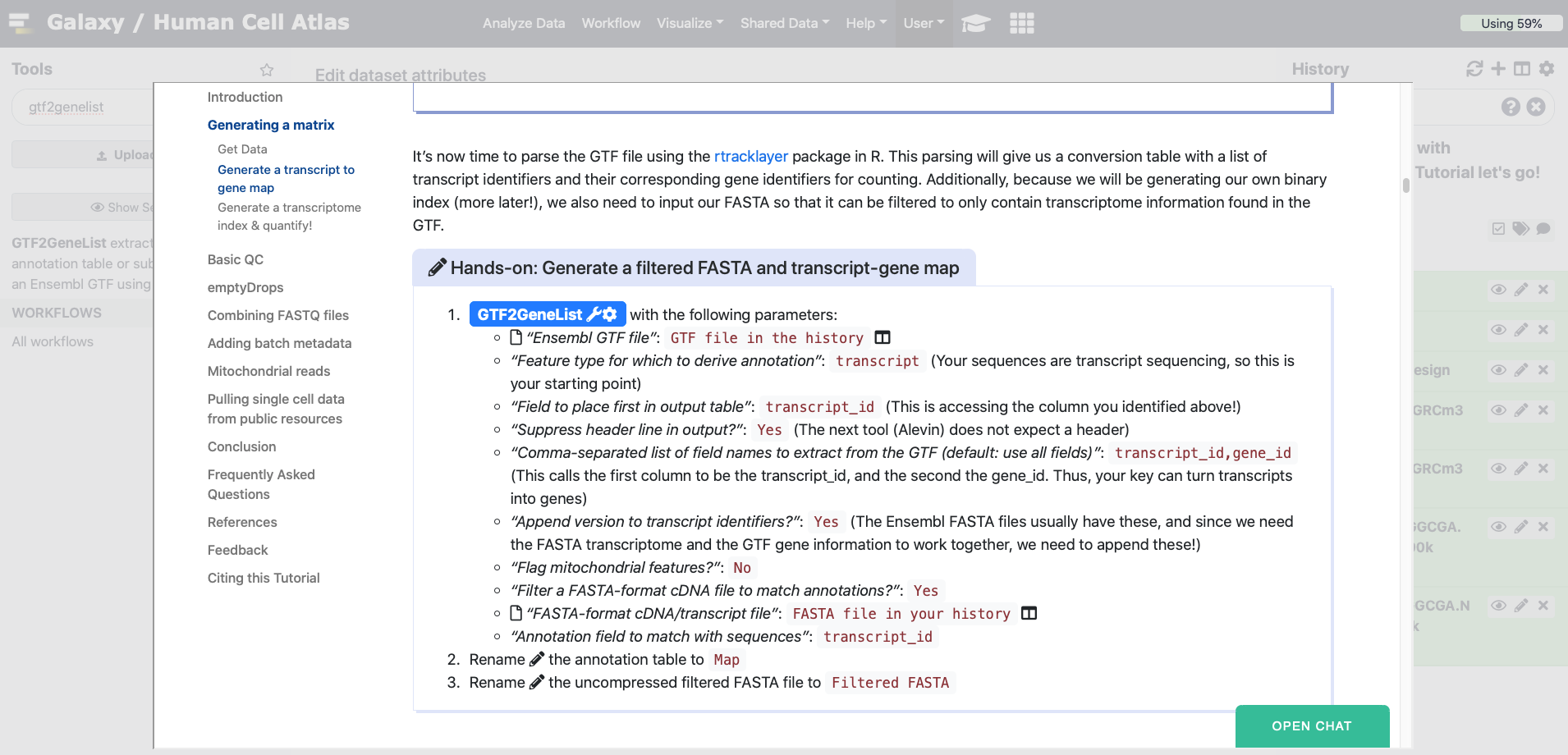
It’s now time to parse the GTF file using the rtracklayer package in R. This parsing will give us a conversion table with a list of transcript identifiers and their corresponding gene identifiers for counting. Additionally, because we will be generating our own binary index (more later!), we also need to input our FASTA so that it can be filtered to only contain transcriptome information found in the GTF.
Tip: Using tutorial mode
Tools are frequently updated to new versions. Your Galaxy may have multiple versions of the same tool available. By default, you will be shown the latest version of the tool. This may NOT be the same tool used in the tutorial you are accessing. Furthermore, if you use a newer tool in one step, and try using an older tool in the next step… this may fail! To ensure you use the same tool versions of a given tutorial, use the Tutorial mode feature.
- Open your Galaxy server
- Click on the curriculum icon on the top menu, this will open the GTN inside Galaxy.
- Navigate to your tutorial
- Tool names in tutorials will be blue buttons that open the correct tool for you
- Note: this does not work for all tutorials (yet)
hands_on Hands-on: Generate a filtered FASTA and transcript-gene map
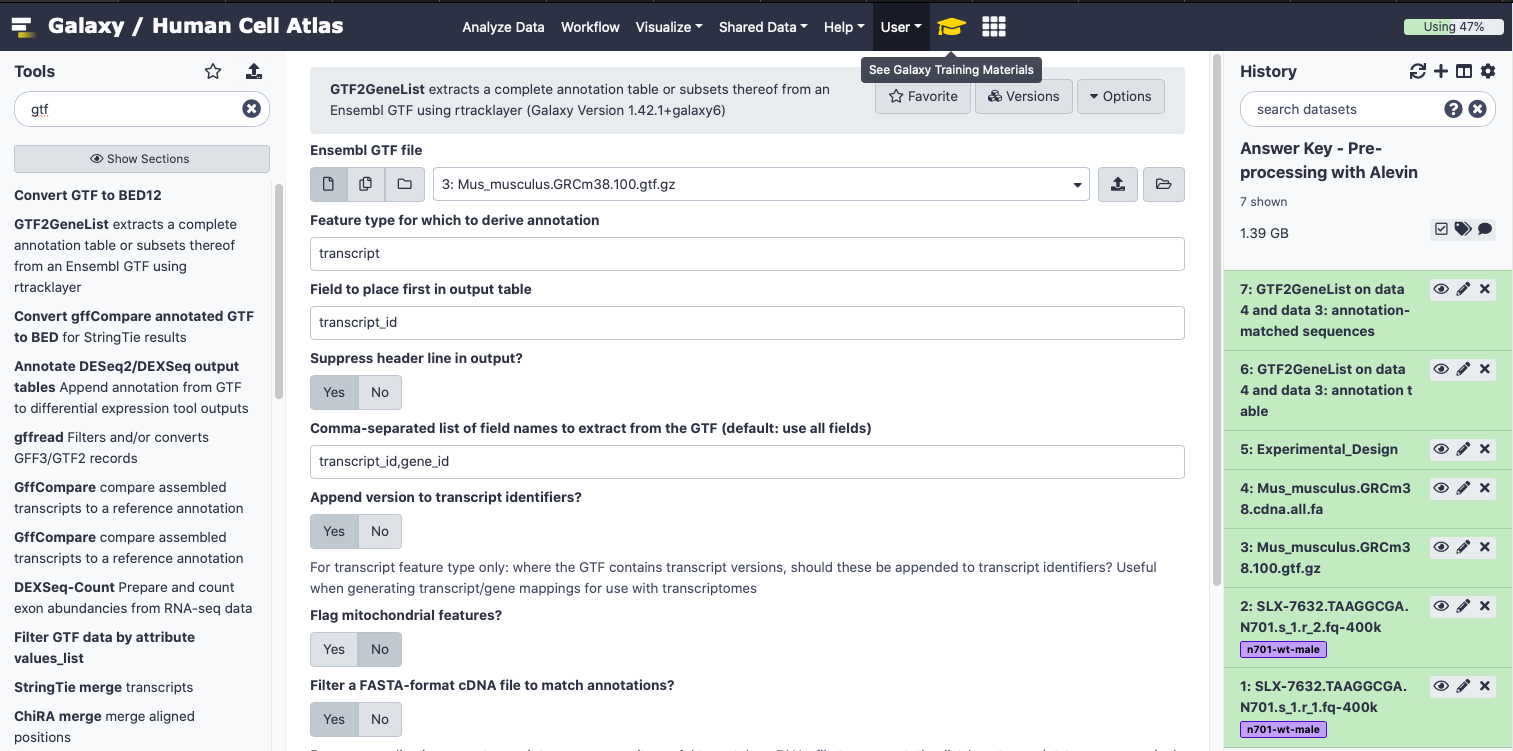
- GTF2GeneList Tool: toolshed.g2.bx.psu.edu/repos/ebi-gxa/gtf2gene_list/_ensembl_gtf2gene_list/1.42.1+galaxy6 with the following parameters:
- param-file “Ensembl GTF file”:
GTF file in the historygalaxy-history- “Feature type for which to derive annotation”:
transcript(Your sequences are transcript sequencing, so this is your starting point)- “Field to place first in output table”:
transcript_id(This is accessing the column you identified above!)- “Suppress header line in output?”:
Yes(The next tool (Alevin) does not expect a header)- “Comma-separated list of field names to extract from the GTF (default: use all fields)”:
transcript_id,gene_id(This calls the first column to be the transcript_id, and the second the gene_id. Thus, your key can turn transcripts into genes)- “Append version to transcript identifiers?”:
Yes(The Ensembl FASTA files usually have these, and since we need the FASTA transcriptome and the GTF gene information to work together, we need to append these!)- “Flag mitochondrial features?”:
No- “Filter a FASTA-format cDNA file to match annotations?”:
Yes- param-file “FASTA-format cDNA/transcript file”:
FASTA file in your historygalaxy-history- “Annotation field to match with sequences”:
transcript_idRename galaxy-pencil the annotation table to
Map- Rename galaxy-pencil the uncompressed filtered FASTA file to
Filtered FASTA
Generate a transcriptome index & quantify!
Alevin collapses the steps involved in dealing with dscRNA-seq into a single process. Such tools need to compare the sequences in your sample to a reference containing all the likely transcript sequences (a ‘transcriptome’). This will contain the biological transcript sequences known for a given species, and perhaps also technical sequences such as ‘spike ins’ if you have those.
details How does Alevin work?
To be able to search a transcriptome quickly, Alevin needs to convert the text (FASTA) format sequences into something it can search quickly, called an ‘index’. The index is in a binary rather than human-readable format, but allows fast lookup by Alevin. Because the types of biological and technical sequences we need to include in the index can vary between experiments, and because we often want to use the most up-to-date reference sequences from Ensembl or NCBI, we can end up re-making the indices quite often. Making these indices is time-consuming! Have a look at the uncompressed FASTA to see what it starts with.
We now have:
- Barcode/ UMI reads
- cDNA reads
- transcript/ gene mapping
- filtered FASTA
We can now run Alevin. In some public instances, Alevin won’t show up if you search for it. Instead, you have to click the Single Cell tab at the left and scroll down to the Alevin tool. Tip: If you click the tools from the tutorial option within Galaxy, you’ll always have the correct version of the tool! In this case, it is: (Galaxy Version 1.3.0+galaxy2) - it should be default. If not, click ‘Versions’ and choose that version.
hands_on Hands-on: Running Alevin
Alevin Tool: toolshed.g2.bx.psu.edu/repos/bgruening/alevin/alevin/1.3.0+galaxy2
question Questions
Try to fill in the parameters of Alevin using what you know!
tip Tip: Strandedness?
The Salmon documentation on ‘Fragment Library Types’ and running the Alevin command (salmon.readthedocs.io/en/latest/library_type.html and salmon.readthedocs.io/en/latest/alevin.html) will help here, although keep in mind the image there is drawn with the RNA 5’ on top, whereas in this scRNA-seq protocol, the polyA is captured by its 3’ tail and thus effectively the bottom or reverse strand…)
solution Solution
- “Select a reference transcriptome from your history or use a built-in index?”:
Use one from the history
- You are going to generate the binary index using your filtered FASTA!
- param-file “Transcripts FASTA file”:
Filtered FASTA- “Single or paired-end reads?”:
Paired-end- param-file “file1”:
N701-Read1- param-file “file2”:
N701-Read2- “Relative orientation of reads within a pair”:
Mates are oriented towards each other (IR)- “Specify the strandedness of the reads”:
read comes from the reverse strand (SR)- “Protocol”:
DropSeq Single Cell protocol- param-file “Transcript to gene map file”:
Map- “Retrieve all output files”:
Yes- In “Optional commands”:
- “dumpFeatures”:
Yes- “dumpMTX”:
Yes
comment What if I’m running a 10x sample?
The main parameter that needs changing for a 10X Chromium sample is the ‘Protocol’ parameter of Alevin. Just select the correct 10x Chemistry there instead.
This tool will take a while to run. Alevin produces many file outputs, not all of which we’ll use. You can refer to the Alevin documentation if you’re curious what they all are, but we’re most interested in is:
- the matrix itself (quants_mat.mtx.gz - the count by gene and cell)
- the row (cell/ barcode) identifiers (quants_mat_rows.txt) and
- the column (gene) labels (quants_mat_cols.txt).
This is the matrix market (MTX) format.
question Questions
After you’ve run Alevin, galaxy-eye look through all the different files. Can you find:
- The Mapping Rate?
- How many cells are present in the matrix output?
solution Solution
- Inspect galaxy-eye the file param-file meta_info.json. You can see the mapping rate is a paltry
24.75%. This is a terrible mapping rate. Why might this be? Remember this was downsampled, and specifically by taking only the last 400,000 reads of the FASTQ file. The overall mapping rate of the file is more like 50%, which is still quite poor, but for early Drop-Seq samples and single-cell data in general, you might expect a slightly poorer mapping rate. 10x samples are much better these days! This is real data, not test data, after all!- Inspect galaxy-eye the file param-file ‘quants_mat_rows.txt’, and you can see it has
2163lines. The rows refer to the cells in the cell x gene matrix. According to this (rough) estimate, your sample has 2163 cells in it!
warning Warning!: Choose the appropriate input going forward!
Make certain to use quants_mat.mtx.gz and NOT quants_tier.mtx.gz going forward.
congratulations Congratulations - you’ve made an expression matrix! We could almost stop here. But it’s sensible to do some basic QC, and one of the things we can do is look at a barcode rank plot.
Basic QC
The question we’re looking to answer here, is: “do we have mostly a have a single cell per droplet”? That’s what experimenters are normally aiming for, but it’s not entirely straightforward to get exactly one cell per droplet. Sometimes almost no cells make it into droplets, other times we have too many cells in each droplet. At a minimum, we should easily be able to distinguish droplets with cells from those without.
hands_on Hands-on: Generate a raw barcode QC plot
- Droplet barcode rank plot Tool: toolshed.g2.bx.psu.edu/repos/ebi-gxa/droplet_barcode_plot/_dropletBarcodePlot/1.6.1+galaxy2 with the following parameters:
- “Input MTX-format matrix?”:
No- param-file “A two-column tab-delimited file, with barcodes in the first column and frequencies in the second”:
raw_cb_frequencies.txt- “Label to place in plot title”:
Barcode rank plot (raw barcode frequencies)- Rename galaxy-pencil the image output
Barcode Plot - raw barcode frequencies
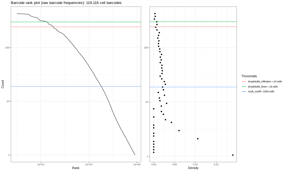
Now, the image generated here (400k) isn’t the most informative - but you are dealing with a fraction of the reads! If you run the total sample (so identical steps above, but with significantly more time!) you’d get the image below.
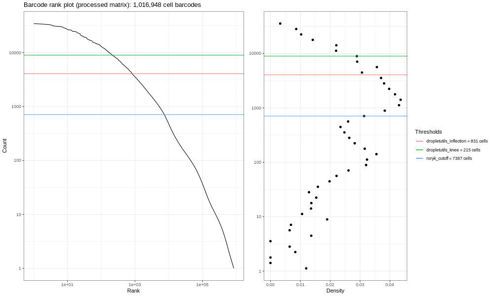
This is our own formulation of the barcode plot based on a discussion we had with community members. The left hand plots with the smooth lines are the main plots, showing the UMI counts for individual cell barcodes ranked from high to low. We expect a sharp drop-off between cell-containing droplets and ones that are empty or contain only cell debris. Now, this data is not an ideal dataset, so for perspective, in an ideal world with a very clean 10x run, data will look a bit more like the following taken from the lung atlas (see the study in Single Cell Expression Atlas here and the project submission here).
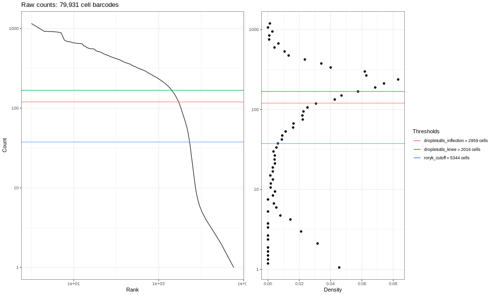
In that plot, you can see the clearer ‘knee’ bend, showing the cut-off between empty droplets and cell-containing droplets.
The right hand plots are density plots from the first one, and the thresholds are generated either using dropletUtils or by the method described in the discussion mentioned above. We could use any of these thresholds to select cells, assuming that anything with fewer counts is not a valid cell. By default, Alevin does something similar, and we can learn something about that by plotting just the barcodes Alevin retains.
hands_on Hands-on: Generate Alevin’s barcode QC plot
- Droplet barcode rank plot Tool: toolshed.g2.bx.psu.edu/repos/ebi-gxa/droplet_barcode_plot/_dropletBarcodePlot/1.6.1+galaxy2 with the following parameters:
- “Input MTX-format matrix?”:
Yes- “Matrix-market format matrix file, with cells by column (overrides –barcode-frequencies if supplied)”:
quants_mat.mtx- “For use with –mtx-matrix: force interpretation of matrix to assume cells are by row, rather than by column (default)”:
Yes- “Label to place in plot title”:
Barcode rank plot (Alevin-processed)- “Number of bins used in barcode count frequency distribution”:
50- “Above-baseline multiplier to calculate roryk threshold”:
1.5- Rename galaxy-pencil the image output
Barcode Plot - Alevin processed barcodes
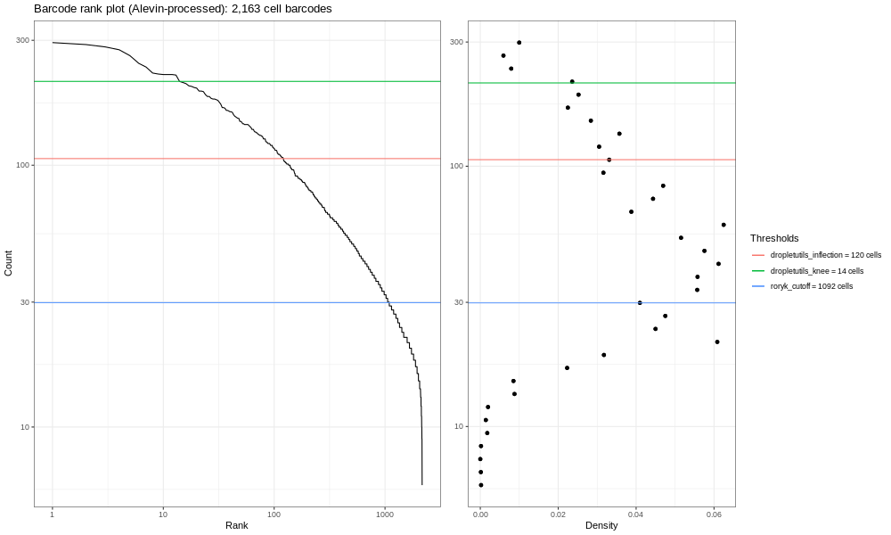
And the full sample looks like:
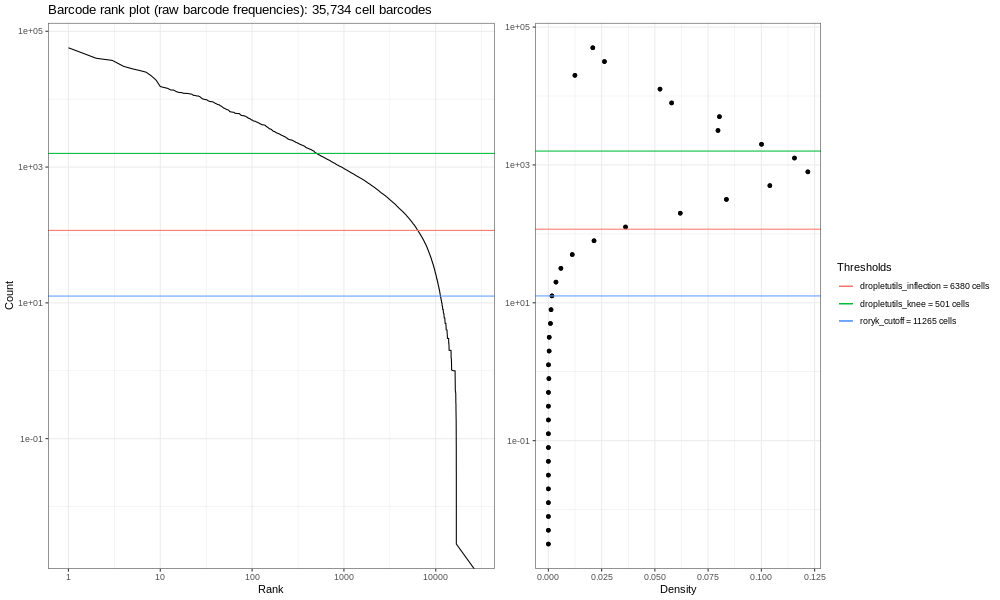
And to round this off, here’s the lung atlas plot.
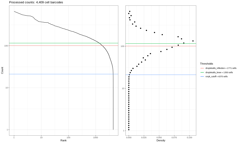
You should see a completely vertical drop-off where Alevin has trunctated the distribution (after excluding any cell barcode that had <10 UMI, Alevin then chose a threshold based off the curve and removed all barcodes with fewer UMIs).
In experiments with relatively simple characteristics, this ‘knee detection’ method works relatively well. But some populations (such as our sample!) present difficulties. For instance, sub-populations of small cells may not be distinguished from empty droplets based purely on counts by barcode. Some libraries produce multiple ‘knees’ for multiple sub-populations. The emptyDrops method has become a popular way of dealing with this. emptyDrops still retains barcodes with very high counts, but also adds in barcodes that can be statistically distinguished from the ambient profiles, even if total counts are similar. In order to ultimately run emptyDrops (or indeed, whatever tool you like that accomplishes biologically relevant thresholding), we first need to re-run Alevin, but prevent it from applying its own less than ideal thresholds.
To use emptyDrops effectively, we need to go back and re-run Alevin, stopping it from applying it’s own thresholds. Click the re-run icon galaxy-refresh on any Alevin output in your history, because almost every parameter is the same as before, except you need to change the following:
Generate an unprocessed matrix in a usable format
hands_on Hands-on: Stopping Alevin from thresholding
- Alevin Tool: toolshed.g2.bx.psu.edu/repos/bgruening/alevin/alevin/1.3.0+galaxy2 (Click re-run on the last Alevin output)
- “Optional commands”
- “keepCBFraction”: ‘1’ - i.e. keep them all!
- “freqThreshold”: ‘3’ - This will only remove cell barcodes with a frequency of less than 3, a low bar to pass but useful way of avoiding processing a bunch of almost certainly empty barcodes
Tip: Re-running a tool
- Expand one of the output datasets of the tool (by clicking on it)
- Click re-run galaxy-refresh the tool
This is useful if you want to run the tool again but with slightly different paramters, or if you just want to check which parameter setting you used.
question Question
How many cells are in the output now?
solution Solution
22539cells are in the quants_mat_rows now! Far more than the Alevin-filtered2163. This needs some serious filtering with EmptyDrops!
Alevin outputs MTX format, which we can pass to the dropletUtils package and run emptyDrops. Unfortunately the matrix is in the wrong orientation for tools expecting files like those produced by 10X software (which dropletUtils does). We need to ‘transform’ the matrix such that cells are in columns and genes are in rows.
warning Be careful!
Don’t mix up files from the different Alevin runs! Use the later run, which has higher numbers in the history!
hands_on Hands-on: Transform matrix
- salmonKallistoMtxTo10x Tool: toolshed.g2.bx.psu.edu/repos/ebi-gxa/salmon_kallisto_mtx_to_10x/_salmon_kallisto_mtx_to_10x/0.0.1+galaxy5 with the following parameters:
- param-file “.mtx-format matrix”:
quants_mat.mtx.gz(output of Alevin tool)- param-file “Tab-delimited genes file”:
quants_mat_cols.txt(output of Alevin tool)- param-file “Tab-delimited barcodes file”:
quants_mat_rows.txt(output of Alevin tool)- Rename galaxy-pencil ‘salmonKallistoMtxTo10x….:genes’ to
Gene table- Rename galaxy-pencil ‘salmonKallistoMtxTo10x….:barcodes’ to
Barcode table- Rename galaxy-pencil ‘salmonKallistoMtxTo10x….:matrix’ to
Matrix table
The output is a matrix in the correct orientation for the rest of our tools. However, our matrix is looking a bit sparse - for instance, click on Gene table. I don’t know about you, but I’d struggle to have a good biological discussion using only Ensembl gene_ids! What I’d really like is the more understandable ‘GAPDH’ or other gene acronym, as well as information on mitochondrial genes so that I can assess if my cells were stressed out or not. In order to prepare our data for emptyDrops, we’re going to combine this information into an object, and it’s easiest to add in that information now.
Adding in Gene metadata
question Question
Where can we find this gene information?
solution Solution
Our old friend the GTF file!
question Question
Which of the ‘attributes’ in the last column of that file contains the gene acronym?
solution Solution
gene_name
We’re now going to re-run galaxy-refresh the tool that extracts information from our GTF file.
hands_on Hands-on: Generate gene information
- GTF2GeneList Tool: toolshed.g2.bx.psu.edu/repos/ebi-gxa/gtf2gene_list/_ensembl_gtf2gene_list/1.42.1+galaxy6 with the following parameters:
- “Feature type for which to derive annotation”:
gene- “Field to place first in output table”:
gene_id- “Suppress header line in output?”:
Yes- “Comma-separated list of field names to extract from the GTF (default: use all fields)”:
gene_id,gene_name,mito- “Append version to transcript identifiers?”:
Yes- “Flag mitochondrial features?”:
Yes- note, this will auto-fill a bunch of acronyms for searching in the GTF for mitochondrial associated genes. This is good!- “Filter a FASTA-format cDNA file to match annotations?”:
No- we don’t need to, we’re done with the FASTA!- Check that the output file type is
tabular. If not, change the file type by clicking the ‘Edit attributes’galaxy-pencil on the dataset in the history (as if you were renaming the file.) Then clickDatatypesand type intabular. ClickChange datatype.)- Rename galaxy-pencil the annotation table to
Gene Information
Inspect galaxy-eye the Gene Information object in the history. Now you have made a new key for gene_id, with gene name and a column of mitochondrial information (false = not mitochondrial, true = mitochondrial). We need to add this information into the salmonKallistoMtxTo10x output ‘Gene table’. But we need to keep ‘Gene table’ in the same order, since it is referenced in the ‘Matrix table’ by row.
hands_on Hands-on: Combine MTX Gene Table with Gene Information
- Join two Datasets Tool: join1 with the following parameters:
- “Join”:
Gene Table- “Using column”:
Column: 1- “with”:
Gene Information- “and column”:
Column: 1- “Keep lines of first input that do not join with second input”:
Yes- “Keep lines of first input that are incomplete”:
Yes- “Fill empty columns”:
No- “Keep the header lines”:
NoIf you inspect galaxy-eye the object, you’ll see we have joined these tables and now have quite a few gene_id repeats. Let’s take those out, while keeping the order of the original ‘Gene Table’.
- Cut columns from a table Tool: Cut1 with the following parameters:
- “Cut columns”:
c1,c4,c5- “Delimited by”:
Tab- “From”: output of Join two Datasets tool
- Rename output
Annotated Gene Table
Inspect galaxy-eye your Annotated Gene Table. That’s more like it! You now have gene_id, gene_name, and mito. Now let’s get back to your journey to emptyDrops and sophisticated thresholding of empty droplets!
emptyDrops
emptyDrops Lun et al. 2019 works with a specific form of R object called a SingleCellExperiment. We need to convert our transformed MTX files into that form, using the DropletUtils Read10x tool:
hands_on Hands-on: Converting to SingleCellExperiment format
- DropletUtils Read10x Tool: toolshed.g2.bx.psu.edu/repos/ebi-gxa/dropletutils_read_10x/dropletutils_read_10x/1.0.3+galaxy2 with the following parameters:
- param-file “Expression matrix in sparse matrix format (.mtx)”:
Matrix table- param-file “Gene Table”:
Annotated Gene Table- param-file “Barcode/cell table”:
Barcode table- “Should metadata file be added?”:
No- Rename galaxy-pencil output:
SCE Object
Fantastic! Now that our matrix is combined into an object, specifically the SingleCellExperiment format, we can now run emptyDrops! Let’s get rid of those background droplets containing no cells!
hands_on Hands-on: Emptydrops
- DropletUtils emptyDrops Tool: toolshed.g2.bx.psu.edu/repos/ebi-gxa/dropletutils_empty_drops/dropletutils_empty_drops/1.0.3+galaxy1 with the following parameters:
- param-file “SingleCellExperiment rdata object”:
SCE Object- “Should barcodes estimated to have no cells be removed from the output object?”:
YesRename galaxy-pencil
serialised SingleCellExperimentoutput asStringent-Object- Rename galaxy-pencil
tabular outputasStringent-Tabular Output
question Question
How many cell barcodes remain after the emptyDrops treatment? Why might that be?
tip Hint
If you click on the
Stringent-Objectin the galaxy-history history, the text in that window says22 barcodesor something similar to that. Why is this so low?? And why might the number be different? Consider…is this a complete set of data?solution Solution
Remember this is a subsampled dataset. If you look carefully at the parameters of emptyDrops, you’ll see it set a minimum threshold at 100 UMI. If you look at the barcode plots above for the 400k read sample, you’ll see this is far too stringent for this subsampled data! To satisfy your curiosity, this minimum threshold would yield
3011barcodes for the total sample. Also, the number may vary slightly as the output depends on a large number of random iterations.
Let’s go back and tweak parameters, re-running the tool with a looser threshold minimum.
details Working in a group? Decision-time!
If you are working in a group, you can now divvy up a decision here with one control and the rest varied numbers so that you can compare results throughout the tutorials.
- Variable: UMI count lower bound
- Control:
5- Everyone else: Consider the droplet barcode rank plots and choose (different) appropriate lower bounds.
hands_on Hands-on: emptyDrops - do-over!
- DropletUtils emptyDrops Tool: toolshed.g2.bx.psu.edu/repos/ebi-gxa/dropletutils_empty_drops/dropletutils_empty_drops/1.0.3+galaxy1 with the following parameters:
- param-file “SingleCellExperiment rdata object”:
SCE Object- “UMI count lower bound”:
5- you can input different numbers here and see what happens!- “Should barcodes estimated to have no cells be removed from the output object?”:
YesRename galaxy-pencil
serialised SingleCellExperimentoutput as<yournumberhere>UMI-Object- Rename galaxy-pencil
tabular outputas<yournumberhere>UMI-Tabular Output
You should now have 111 barcodes! You now have an annotated expression matrix ready to go for further processing and analysis! Well done! However, the next tutorials we will link to use a tool called Scanpy. You need to convert this SingleCellExperiment object into a format called annData, which is a variant of a file format called hdf5.
hands_on Hands-on: Converting to AnnData format
- SCEasy convert Tool: toolshed.g2.bx.psu.edu/repos/ebi-gxa/sceasy_convert/sceasy_convert/0.0.5+galaxy1 with the following parameters:
- “Direction of conversion”:
SingleCellExperiment to AnnData- param-file “Input object in SingleCellExperiment RDS format”:
<yournumberhere>UMI-Object- “Name of the assay to be transferred as main layer”:
counts- Rename galaxy-pencil output
N701-400k-AnnData
congratulations Congrats! Your object is ready to for the scanpy pipeline! You can can check your work against the example history.
However, it may be that you want to combine this object with others like it, for instance, maybe you ran 5 samples, and you are starting with 10 FASTQ files…
Combining FASTQ files
This sample was originally one of seven. So to run the other 12 downsampled FASTQ files, you can use a workflow! Note - the N705 subsample is unluckily largely junk reads, so emptyDrops doesn’t work. Instead, I processed it with Alevin. The total sample runs fine on emptyDrops of course. All these samples are going to take a while, so go and have several cups of tea… Or, better yet, I have run them myself, and plopped them in a new clean history for you to import as a fresh history. Alternatively, you can get data with zenodo.
Data
hands_on Hands-on: Data upload - Combining files
- Create a new history for this tutorial (if you’re not importing the history above)
Import the different AnnData files and the experimental design table from Zenodo
https://zenodo.org/record/4574153/files/Experimental_Design.tabular
https://zenodo.org/record/4574153/files/N701-400k-AnnData.h5ad
https://zenodo.org/record/4574153/files/N702-400k-AnnData.h5ad
https://zenodo.org/record/4574153/files/N703-400k-AnnData.h5ad
https://zenodo.org/record/4574153/files/N704-400k-AnnData.h5ad
https://zenodo.org/record/4574153/files/N705-400k-AnnData.h5ad
https://zenodo.org/record/4574153/files/N706-400k-AnnData.h5ad
https://zenodo.org/record/4574153/files/N707-400k-AnnData.h5ad
Tip: Importing via links
- Copy the link location
Open the Galaxy Upload Manager (galaxy-upload on the top-right of the tool panel)
- Select Paste/Fetch Data
Paste the link into the text field
Press Start
- Close the window
- Rename the datasets
Check that the datatype is
h5ad, otherwise you will need to change each file toh5ad!Tip: Changing the datatype
- Click on the galaxy-pencil pencil icon for the dataset to edit its attributes
- In the central panel, click on the galaxy-chart-select-data Datatypes tab on the top
- Select
datatypes
- tip: you can start typing the datatype into the field to filter the dropdown menu
- Click the Save button
Inspect the galaxy-eye Experimental Design text file. This shows you how each N70X corresponds to a sample, and whether that sample was from a male or female. This will be important metadata to add to our sample, which we will add very similarly to how you added the gene_name and mito metadata above!
Concatenating objects
hands_on Hands-on: Concatenating AnnData objects
- Manipulate AnnData Tool: toolshed.g2.bx.psu.edu/repos/iuc/anndata_manipulate/anndata_manipulate/0.7.5+galaxy0 with the following parameters:
- param-file “Annotated data matrix”:
N701-400k-AnnData- “Function to manipulate the object”: ‘Concatenate along the observations axis’
- param-file “Annotated data matrix to add”: ‘Select all the other matrix files from bottom to top’
- “Join method”:
Intersection of variables- “Key to add the batch annotation to obs”:
batch- “Separator to join the existing index names with the batch category”:
-
Now let’s look at what we’ve done! Unfortunately, AnnData objects are quite complicated, so the galaxy-eye won’t help us too much here. Instead, we’re going to use a tool to look into our object from now on.
hands_on Hands-on: Inspecting AnnData Objects
- Inspect AnnData Tool: toolshed.g2.bx.psu.edu/repos/iuc/anndata_inspect/anndata_inspect/0.7.5+galaxy0 with the following parameters:
- param-file “Annotated data matrix”: output of Manipulate AnnData tool
- “What to inspect?”:
General information about the object- Inspect AnnData Tool: toolshed.g2.bx.psu.edu/repos/iuc/anndata_inspect/anndata_inspect/0.7.5+galaxy0 with the following parameters:
- param-file “Annotated data matrix”: output of Manipulate AnnData tool
- “What to inspect?”:
Key-indexed observations annotation (obs)- Inspect AnnData Tool: toolshed.g2.bx.psu.edu/repos/iuc/anndata_inspect/anndata_inspect/0.7.5+galaxy0 with the following parameters:
- param-file “Annotated data matrix”: output of Manipulate AnnData tool
- “What to inspect?”:
Key-indexed annotation of variables/features (var)
Now have a look at the three tool Inspect AnnData outputs.
question Question
- How many cells do you have now?
- Where is
batchinformation stored?solution Solution
- If you look at the General information tool output, you can see there are now
4079 cells, as the matrix is now 4079 cells x 35734 genes. You can see this as well in the obs tool (cells) and var tool (genes) file sizes.- Under Key-indexed observations annotation (obs). Different version of the Manipulate tool will put the
batchcolumns in different locations. The tool version in this course has the9thcolumn at the farthest right isbatch. Batch refers to the order in which the matrices were added. The files are added from the bottom of the history upwards, so be careful how you set up your histories when running this!
Adding batch metadata
I set up the example history with the earliest indices at the bottom.
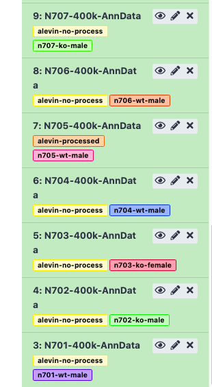
Therefore, when it is all concatenated together, the batch appears as follows:
| Index | Batch | Genotype | Sex |
|---|---|---|---|
| N701 | 0 | wildtype | male |
| N702 | 1 | knockout | male |
| N703 | 2 | knockout | female |
| N704 | 3 | wildtype | male |
| N705 | 4 | wildtype | male |
| N706 | 5 | wildtype | male |
| N707 | 6 | knockout | male |
If you used Zenodo to import files, they may not have imported in order (i.e. N701 to N707, ascending). In that case, you will need to tweak the parameters of the next tools appropriately to label your batches correctly!
The two critical pieces of metadata in this experiment are sex and genotype. I will later want to color my cell plots by these parameters, so I want to add them in now!
hands_on Hands-on: Labelling sex
- Replace Text in a specific column Tool: toolshed.g2.bx.psu.edu/repos/bgruening/text_processing/tp_replace_in_column/1.1.3 with the following parameters:
- param-file “File to process”: output of Inspect AnnData: Key-indexed observations annotation (obs) tool)
“1. Replacement”
- “in column”:
Column: 9- or whichever columnbatchis in- “Find pattern”:
0|1|3|4|5|6- “Replace with”:
male- + Insert Replacement
“2. Replacement”
- “in column”:
Column: 9- “Find pattern”:
2- “Replace with”:
female- + Insert Replacement
“3. Replacement”
- “in column”:
Column: 9- “Find pattern”:
batch- “Replace with”:
sexNow we want only the column containing the sex information - we will ultimately add this into the cell annotation in the AnnData object.
- Cut columns from a table Tool: Cut1 with the following parameters:
- “Cut columns”:
c9- “Delimited by”:
Tab- % icon param-file %} “From”: output of Replace text tool
- Rename galaxy-pencil output
Sex metadata
That was so fun, let’s do it all again but for genotype!
hands_on Hands-on: Labelling genotype
- Replace Text in a specific column Tool: toolshed.g2.bx.psu.edu/repos/bgruening/text_processing/tp_replace_in_column/1.1.3 with the following parameters:
- param-file “File to process”: output of Inspect AnnData: Key-indexed observations annotation (obs) tool
“1. Replacement”
- “in column”:
Column: 9- “Find pattern”:
0|3|4|5- “Replace with”:
wildtype- + Insert Replacement
“2. Replacement”
- “in column”:
Column: 9- “Find pattern”:
1|2|6- “Replace with”:
knockout- + Insert Replacement
“3. Replacement”
- “in column”:
Column: 9- “Find pattern”:
batch- “Replace with”:
genotypeNow we want only the column containing the genotype information - we will ultimately add this into the cell annotation in the AnnData object.
- Cut columns from a table Tool: Cut1 with the following parameters:
- “Cut columns”:
c9- “Delimited by”:
Tab- param-file “From”: output of Replace text tool
- Rename galaxy-pencil output
Genotype metadata
You might want to do this with all sorts of different metadata - which labs handled the samples, which days they were run, etc. Once you’ve added all your metadata columns, we can add them together before plugging them into the AnnData object itself.
hands_on Hands-on: Combining metadata columns
- Paste two files side by side Tool: Paste1 with the following parameters:
- param-file “Paste”:
Genotype metadata- param-file “and”:
Sex metadata- “Delimit by”:
Tab- Rename galaxy-pencil output
Cell Metadata
Let’s add it to the AnnData object!
hands_on Hands-on: Adding metadata to AnnData object
- Manipulate AnnData Tool: toolshed.g2.bx.psu.edu/repos/iuc/anndata_manipulate/anndata_manipulate/0.7.5+galaxy0 with the following parameters:
- param-file “Annotated data matrix”: output of previous Manipulate AnnData tool
- “Function to manipulate the object”:
Add new annotation(s) for observations or variables- “What to annotate?”:
Observations (obs)`- param-file “Table with new annotations”:
Cell Metadata
Woohoo! We’re there! You can run an Inspect AnnData to check now, but I want to clean up this AnnData object just a bit more first. It would be a lot nicer if ‘batch’ meant something, rather than ‘the order in which the Manipulate AnnData tool added my datasets’.
hands_on Hands-on: Labelling batches
- Manipulate AnnData Tool: toolshed.g2.bx.psu.edu/repos/iuc/anndata_manipulate/anndata_manipulate/0.7.5+galaxy0 with the following parameters:
- param-file “Annotated data matrix”: output of Manipulate AnnData - Add new annotations tool
- “Function to manipulate the object”:
Rename categories of annotation- “Key for observations or variables annotation”:
batch- “Comma-separated list of new categories”:
N701,N702,N703,N704,N705,N706,N707
Huzzah! We are JUST about there. However, while we’ve been focussing on our cell metadata (sample, batch, genotype, etc.) to relabel the ‘observations’ in our object…
Mitochondrial reads
Do you remember when we mentioned mitochondria early on in this tutorial? And how often in single cell samples, mitochondrial RNA is often an indicator of stress during dissociation? We should probably do something with our column of true/false in the gene annotation that tells us information about the cells. You will need to do this whether you have combined FASTQ files or are analysing just one (and thus skipping sections 4 & 5).
hands_on Hands-on: Calculating mitochondrial RNA in cells
- AnnData Operations Tool: toolshed.g2.bx.psu.edu/repos/ebi-gxa/anndata_ops/anndata_ops/0.0.3+galaxy1 with the following parameters:
- param-file “Input object in hdf5 AnnData format”: output of Manipulate AnnData - Rename categories tool
- “Format of output object”:
AnnData format- “Copy AnnData to .raw”:
No- “Gene symbols field in AnnData”:
NA.- “Flag genes that start with these names”:
Insert Flag genes that start with these names- “Starts with”:
True- “Var name”:
mito- “Number of top genes”:
50
congratulationsWell done! I strongly suggest have a play with the Inspect AnnData tool on your final Pre-processed object to see the wealth of information that has been added. You are now ready to move along to further filtering! There is a cheat that may save you time in the future though…
Pulling single cell data from public resources
If you happen to be interested in analysing publicly available data, particularly from the Single Cell Expression Atlas, you may be interested in the following tool Moreno et al. 2020 which rather skips forward all these steps in one! For this tutorial, the dataset can be seen here with experiment id of E-MTAB-6945.
hands_on Hands-on: Retrieving data from Single Cell Expression Atlas
- EBI SCXA Data Retrieval Tool: toolshed.g2.bx.psu.edu/repos/ebi-gxa/retrieve_scxa/retrieve_scxa/v0.0.2+galaxy2 with the following parameters:
- “SC-Atlas experiment accession”:
E-MTAB-6945- “Choose the type of matrix to download”:
Raw filtered countsNow we need to transform this into an AnnData objects
- Scanpy Read10x Tool: toolshed.g2.bx.psu.edu/repos/ebi-gxa/scanpy_read_10x/scanpy_read_10x/1.6.0+galaxy0 with the following parameters:
- “Expression matrix in sparse matrix format (.mtx)”:
EBI SCXA Data Retrieval on E-MTAB-6945 matrix.mtx (Raw filtered counts)- “Gene table”:
EBI SCXA Data Retrieval on E-MTAB-6945 genes.tsv (Raw filtered counts)- “Barcode/cell table”:
EBI SCXA Data Retrieval on E-MTAB-6945 barcodes.tsv (Raw filtered counts)- “Cell metadata table”:
EBI SCXA Data Retrieval on E-MTAB-6945 exp_design.tsv
It’s important to note that this matrix is processed somewhat through the SCXA pipeline, which is quite similar to this tutorial, and it contains any and all metadata provided by their pipeline as well as the authors (for instance, more cell or gene annotations).
Conclusion
You’ve reached the end of this session!
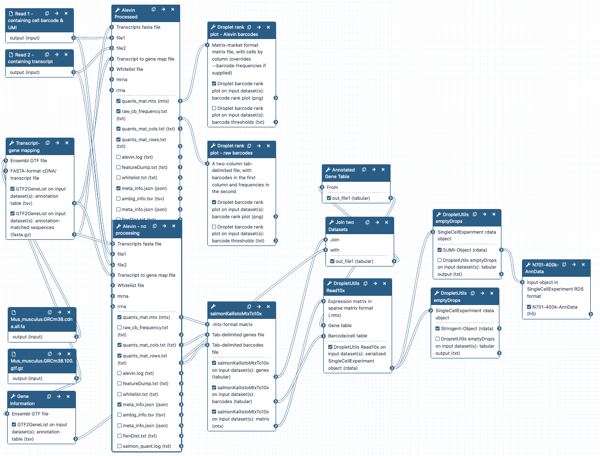
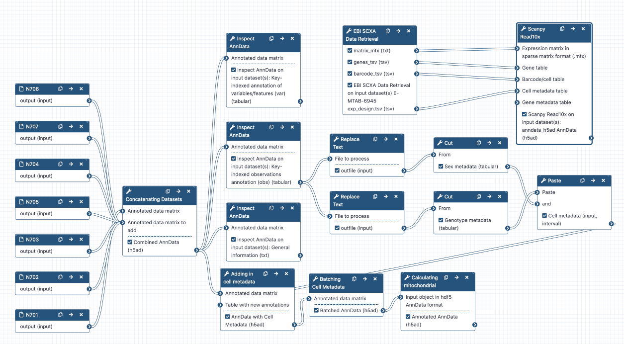
You may be interested in seeing an example history and Part 2 workflow. Note that the workflow will require changing of the column containing the batch metadata depending on how you are running it. The final object containing all the reads can be found in here.
We have:
- Taken raw read data and annotations and necessary input files for quantification.
- Run Alevin in two different parameterisations, both allowing Alevin to make its own calls on what constitutes empty droplets, and applying emptyDrops instead.
- Deployed barcode rank plots as a way of quickly assessing the signal present in droplet datasets.
- Applied the necessary conversion to pass these data to downstream processes.
- Retrieved partially analysed data from the Single Cell Expression Atlas
To discuss with like-minded scientists, join our Gitter channel for all things Galaxy-single cell!
Key points
Create a scanpy-accessible AnnData object from FASTQ files, including relevant cell and gene metadata
Combine multiple samples and label according to study design
Frequently Asked Questions
Have questions about this tutorial? Check out the tutorial FAQ page or the FAQ page for the Transcriptomics topic to see if your question is listed there. If not, please ask your question on the GTN Gitter Channel or the Galaxy Help ForumUseful literature
Further information, including links to documentation and original publications, regarding the tools, analysis techniques and the interpretation of results described in this tutorial can be found here.
References
- Bacon, W. A., R. S. Hamilton, Z. Yu, J. Kieckbusch, D. Hawkes et al., 2018 Single-Cell Analysis Identifies Thymic Maturation Delay in Growth-Restricted Neonatal Mice. Frontiers in Immunology 9: 10.3389/fimmu.2018.02523
- Lun, A., S. Riesenfeld, T. Andrews, T. Dao, T. Gomes et al., 2019 EmptyDrops: Distinguishing cells from empty droplets in droplet-based single-cell RNA sequencing data. Genome Biology 20: 63. 10.1186/s13059-019-1662-y
- Srivastava, A., L. Malik, T. Smith, I. Sudbery, and R. Patro, 2019 Alevin efficiently estimates accurate gene abundances from dscRNA-seq data. Genome Biology 20: 10.1186/s13059-019-1670-y
- Moreno, P., N. Huang, J. R. Manning, S. Mohammed, A. Solovyev et al., 2020 User-friendly, scalable tools and workflows for single-cell analysis. bioRxiv. 10.1101/2020.04.08.032698 https://www.biorxiv.org/content/early/2020/04/09/2020.04.08.032698
Feedback
Did you use this material as an instructor? Feel free to give us feedback on how it went.
Did you use this material as a learner or student? Click the form below to leave feedback.
Citing this Tutorial
- Wendi Bacon, Jonathan Manning, 2022 Generating a single cell matrix using Alevin (Galaxy Training Materials). https://training.galaxyproject.org/training-material/topics/transcriptomics/tutorials/droplet-quantification-preprocessing/tutorial.html Online; accessed TODAY
- Batut et al., 2018 Community-Driven Data Analysis Training for Biology Cell Systems 10.1016/j.cels.2018.05.012
details BibTeX
@misc{transcriptomics-droplet-quantification-preprocessing,
author = "Wendi Bacon and Jonathan Manning",
title = "Generating a single cell matrix using Alevin (Galaxy Training Materials)",
year = "2022",
month = "03",
day = "01"
url = "\url{https://training.galaxyproject.org/training-material/topics/transcriptomics/tutorials/droplet-quantification-preprocessing/tutorial.html}",
note = "[Online; accessed TODAY]"
}
@article{Batut_2018,
    doi = {10.1016/j.cels.2018.05.012},
    url = {https://doi.org/10.1016%2Fj.cels.2018.05.012},
    year = 2018,
    month = {jun},
    publisher = {Elsevier {BV}},
    volume = {6},
    number = {6},
    pages = {752--758.e1},
    author = {B{\'{e}}r{\'{e}}nice Batut and Saskia Hiltemann and Andrea Bagnacani and Dannon Baker and Vivek Bhardwaj and Clemens Blank and Anthony Bretaudeau and Loraine Brillet-Gu{\'{e}}guen and Martin {\v{C}}ech and John Chilton and Dave Clements and Olivia Doppelt-Azeroual and Anika Erxleben and Mallory Ann Freeberg and Simon Gladman and Youri Hoogstrate and Hans-Rudolf Hotz and Torsten Houwaart and Pratik Jagtap and Delphine Larivi{\`{e}}re and Gildas Le Corguill{\'{e}} and Thomas Manke and Fabien Mareuil and Fidel Ram{\'{\i}}rez and Devon Ryan and Florian Christoph Sigloch and Nicola Soranzo and Joachim Wolff and Pavankumar Videm and Markus Wolfien and Aisanjiang Wubuli and Dilmurat Yusuf and James Taylor and Rolf Backofen and Anton Nekrutenko and Björn Grüning},
    title = {Community-Driven Data Analysis Training for Biology},
    journal = {Cell Systems}
}
 Questions:
