Deep Learning (Part 2) - Recurrent neural networks (RNN)
Overview
Questions:Objectives:
What is a recurrent neural network (RNN)?
What are some applications of RNN?
Requirements:
Understand the difference between feedforward neural networks (FNN) and RNN
Learn various RNN types and architectures
Learn how to create a neural network using Galaxy’s deep learning tools
Solve a sentiment analysis problem on IMDB movie review dataset using RNN in Galaxy
- Introduction to Galaxy Analyses
- Statistics and machine learning
- Introduction to deep learning: tutorial hands-on
- Deep Learning (Part 1) - Feedforward neural networks (FNN): slides slides - tutorial hands-on
Time estimation: 2 hoursSupporting Materials:Last modification: May 21, 2021
Introduction
Artificial neural networks are a machine learning discipline roughly inspired by how neurons in a human brain work. In the past decade, there has been a huge resurgence of neural networks thanks to the vast availability of data and enormous increases in computing capacity (Successfully training complex neural networks in some domains requires lots of data and compute capacity). There are various types of neural networks (Feedforward, recurrent, etc). In this tutorial, we discuss recurrent neural networks, which model sequential data, and have been successfully applied to language generation, machine translation, speech recognition, image description, and text summarization (Wen et al. 2015, Cho et al. 2014, Lim et al. 2016, Karpathy and Fei-Fei 2017, Li et al. 2017). We then explain how RNN differ from feedforward networks, describe various RNN architectures and solve a sentiment analysis problem using RNN in Galaxy.
Agenda
In this tutorial, we will cover:
Review of feedforward neural networks (FNN)
In feedforward neural networks (FNN) a single training example is presented to the network, after which the the network generates an output. For example, a lung X-ray image is passed to a FNN, and the network predicts tumor or no tumor. By contrast, in RNN a training example is a sequence, which is presented to the network one at a time. For example, a sequence of English words is passed to a RNN, one at a time, and the network generates a sequence of Persian words, one at a time. RNN handle sequential data, whether its temporal or ordinal.
Single layer FNN
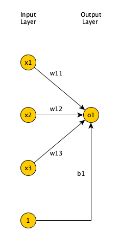
Figure 1 shows a single layer FNN, where the input is 3 dimensional. Each input field is multiplied by a weight. Afterwards, the results are summed up, along with a bias, and passed to an activation function.

The activation function can have many forms (sigmoid, tanh, ReLU, linear, step function, sign function, etc.). Output layer neurons usually have sigmoid or tanh functions. For more information on the listed activation functions, please refer to Nwankpa et al. 2018.

Multi-layer FNN
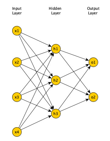
Minsky and Papert showed that a single layer FNN cannot solve problems in which the data is not linearly separable, such as the XOR problem (Newell 1969). Adding one (or more) hidden layers to FNN enables it to solve problems in which data is non-linearly separable. Per Universal Approximation Theorem, a FNN with one hidden layer can represent any function (Cybenko 1989), although in practice training such a model is very difficult (if not impossible), hence, we usually add multiple hidden layers to solve complex problems.
Learning algorithm
In supervised learning, we are given a set of input-output pairs, called the training set. Given the training set, the learning algorithm (iteratively) adjusts the model parameters, so that the model can accurately map inputs to outputs. We usually have another set of input-output pairs, called the test set, which is not used by the learning algorithm. When the learning algorithm completes, we assess the learned model by providing the test set inputs to the model and comparing the model outputs to test set outputs. We need to define a loss function to objectively measure how much the model output is off of the expected output. For classification problems we use the cross entropy loss function.

The loss function is calculated for each input-output pair in the training set. The average of the calculated loss functions for all training set input-output pairs is called the Cost function. The goal of the learning algorithm is to minimize the cost function. The cost function is a function of network weights and biases of all neurons in all layers. The backpropagation learning algorithm Rumelhart et al. 1986 iteratively computes the gradient of cost function relative to each weight and bias, then updates the weights and biases in the opposite direction of the gradient, to find the local minimum.

Recurrent neural networks
Unlike FNN, in RNN the output of the network at time t is used as network input at time t+1. RNN handle sequential data (e.g. temporal or ordinal).
Possible RNN inputs/outputs
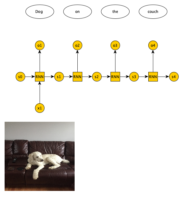
There are 4 possible input/output combinations for RNN and each have a specific application. One-to-one is basically a FNN. One-to-many, where we have one input and a variable number of outputs. One example application is image captioning, where a single image is provided as input and a variable number of words (which caption the image) is returned as output (See Figure 7).
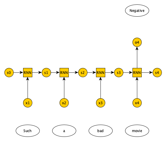
Many-to-one RNN, on the other hand, have a variable number of inputs and a single output. One example application is document sentiment classification, where a variable number of words in a document are presented as input, and a single output predicts whether the document has a positive or negative sentiment regarding a topic (See Figure 8).
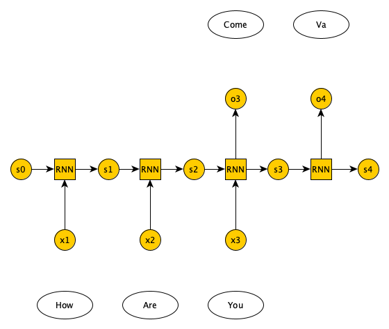
There are two types of many-to-many RNN. One in which the number of inputs and outputs match, e.g., in labeling the video frames the number of frames matches the number of labels, and the other in which the number of inputs and outputs do not match, e.g., in language translation we pass in n words in English and get m words in Italian (See Figure 9).
RNN architectures
Mainly, there are three types of RNN: 1) Vanilla RNN, 2) LSTM (Hochreiter and Schmidhuber 1997), and 3) GRU (Cho et al. 2014). A Vanilla RNN, simply combines the state information from the previous timestamp with the input from the current timestamp to generate the state information and output for current timestamp. The problem with Vanilla RNN is that training deep RNN networks is impossible due to the vanishing gradient problem. Basically, weights/biases are updated according to the gradient of the loss functions relative to the weights/biases. The gradients are calculated recursively from the output layer towards the input layer (Hence, the name backpropagation). The gradient of the input layer is the product of the gradient of the subsequent layers. If those gradients are small, the gradient of the input layer (which is the product of multiple small values) will very small, resulting in very small updates to weights/biases of the initial layers of the RNN, effectively halting the learning process.
LSTM and GRU are two RNN architectures that address vanishing gradient problem. Full description of LSTM/GRU is beyond the scope of this tutorial (Please refer to Hochreiter and Schmidhuber 1997 and Cho et al. 2014), but in a nutshell both LSTM and GRU use gates such that the weights/biases updates in previous layers are calculated via a series of additions (not multiplications). Hence, these architectures can learn even when the RNN has hundreds or thousands of layers.
Text representation schemes
In this tutorial we perform sentiment analysis on IMDB (https://www.imdb.com/) movie reviews dataset (Maas et al. 2011). We train our RNN on the training dataset, which is made up of 25000 movie reviews, some positive and some negative. We then test our RNN on the test set, which is also made up of 25000 movie reviews, again some positive and some negative. The training and test sets have no overlap. Since we are dealing with text data, it’s a good idea to review various mechanisms for representing text data. Before that, we are going to briefly discuss how to preprocess text documents.
Text preprocessing
The first step is to tokenize a document, i.e., break it down into words. Next, we remove the punctuation marks, URLs, and stop words – words like ‘a’, ‘of’, ‘the’, etc. that happen frequently in all documents and do not have much value in discriminating between documents. Next, we normalize the text, e.g., replace ‘brb’ with ‘Be right back’, etc. Then, We then run the spell checker to fix typos and also make all words lowercase. Next, we perform stemming or lemmatization. Basically, if we have words like ‘organizer’, ‘organize’, ‘organized’, and ‘organization’ we want to reduce all of them to a single word. Stemming cuts the end of these words to come up with a single root (e.g., ‘organiz’). The root may not be an actual word. Lemmatization is smarter in that it reduces the word variants to a root that is actually a word (e.g., ‘organize’). All of these steps help reduce the number of features in feature vector of a document and should make the training of our model faster/easier.
For this introductory tutorial, we do minimal text preprocessing. We ignore the top 50 words in IMDB reviews (mostly stop words) and include the next 10,000 words in our dataset. Reviews are limited to 500 words. They are trimmed if they are longer and padded if they are shorter.
Bag of words and TF-IDF
If you don’t care about the order of the words in a document, you can use bag of words (BoW) or term frequency inverse document frequency (TF-IDF). In these models we have a 2 dimensional array. The rows represent the documents (in our example, the movie reviews) and the columns represent the words in our vocabulary (all the unique words in all the documents). If a word is not present in a document, we have a zero at the corresponding row and column as the entry. If a word is present in the document, we have a one as the entry – Alternatively, we could use the word count or frequency.

Suppose we have the following 2 documents: 1) Magic passed the basketball to Kareem, and 2) Lebron stole the basketball from Curry. The BoW representation of these documents is given in Figure 10.
BoW’s advantage is its simplicity, yet it does not take into account the rarity of a word across documents, which unlike common words are important for document classification.
In TF-IDF, similar to BoW we have an entry for each document-word pair. In TD-IDF, the entry is the product of 1) Term frequency, the frequency of a word in a document, and 2) Inverse document frequency, the inverse of the number of documents that have the word divided by the total number of documents (we usually use logarithm of the IDF).
TF-IDF takes into account the rarity of a word across documents, but like BoW does not capture word order or word meaning in documents. BoW and TF-IDF are suitable representations for when word order is not important. They are used in document classification problems like spam detection.
One hot encoding (OHE)
OHE is a technique to convert categorical variables such as words into a vector. Suppose our vocabulary has 3 words: orange, apple, banana. Each word for this vocabulary is represented by a vector of size 3. Orange is represented by a vector whose first element is 1 and other elements are 0; Apple is represented by a vector whose second element is 1 and other elements are 0; And banana is represented by a vector whose third element is 1 and other elements are 0. As you can see only one element in the vector is 1 and the rest are 0’s. The same concept applies if the size of the vocabulary is N.

The problem with OHE is that for very large vocabulary sizes (say, 100,000 words) it requires tremendous amount of storage. Also, it has no concept of word similarity.
Word2Vec
In Word2Vec, each word is represented as an n dimensional vector (n being much smaller than vocabulary size), such that the words that have similar meanings are closer to each other in the vector space, and words that don’t have a similar meaning are farther apart. Words are considered to have a similar meaning if they co-occur often in documents. There are 2 Word2Vec architectures, one that predicts the probability of a word given the surrounding words (Continuous BOW), and one that given a word predicts the probability of the surrounding words (Continuous skip-gram).
In this tutorial, we find an n dimensional representation of the IMDB movie review words, not based on word meanings, but based on how they improve the sentiment classification task. The n dimensional representation is learned by the learning algorithm, simply by reducing the cost function via backpropagation.
Get Data
hands_on Hands-on: Data upload
Create a new history for this tutorial
Tip: Creating a new history
Click the new-history icon at the top of the history panel.
If the new-history is missing:
- Click on the galaxy-gear icon (History options) on the top of the history panel
- Select the option Create New from the menu
Import the files from Zenodo or from the shared data library
https://zenodo.org/record/4477881/files/X_test.tsv
https://zenodo.org/record/4477881/files/X_train.tsv
https://zenodo.org/record/4477881/files/y_test.tsv
https://zenodo.org/record/4477881/files/y_train.tsv
Tip: Importing via links
- Copy the link location
Open the Galaxy Upload Manager (galaxy-upload on the top-right of the tool panel)
- Select Paste/Fetch Data
Paste the link into the text field
Press Start
- Close the window
Tip: Importing data from a data library
As an alternative to uploading the data from a URL or your computer, the files may also have been made available from a shared data library:
- Go into Shared data (top panel) then Data libraries
- Navigate to the correct folder as indicated by your instructor
- Select the desired files
- Click on the To History button near the top and select as Datasets from the dropdown menu
- In the pop-up window, select the history you want to import the files to (or create a new one)
- Click on Import
Rename the datasets as
X_test,X_train,y_test, andy_trainrespectively.Tip: Renaming a dataset
- Click on the galaxy-pencil pencil icon for the dataset to edit its attributes
- In the central panel, change the Name field
- Click the Save button
Check that the datatype of all the four datasets is
tabular. If not, change the dataset’s datatype to tabular.Tip: Changing the datatype
- Click on the galaxy-pencil pencil icon for the dataset to edit its attributes
- In the central panel, click on the galaxy-chart-select-data Datatypes tab on the top
- Select
tabular
- tip: you can start typing the datatype into the field to filter the dropdown menu
- Click the Save button
Sentiment Classification of IMDB movie reviews with RNN
In the section, we define a RNN and train it using IMDB movie reviews training dataset. The goal is to learn a model such that given the words in a review we can predict whether the review was positive or negative. We then evaluate the trained RNN on the test dataset and plot the confusion matrix.
Create a deep learning model architecture
hands_on Hands-on: Model config
- Create a deep learning model architecture Tool: toolshed.g2.bx.psu.edu/repos/bgruening/keras_model_config/keras_model_config/0.5.0
- “Select keras model type”:
sequential- “input_shape”:
(500,)- In “LAYER”:
- param-repeat “1: LAYER”:
- “Choose the type of layer”:
Embedding -- Embedding
- “input_dim””:
10000- “output_dim””:
32- param-repeat “2: LAYER”:
- “Choose the type of layer”:
Recurrent -- LSTM
- “units””:
100- param-repeat “3: LAYER”:
- “Choose the type of layer”:
Core -- Dense
- “units”:
1- “Activation function”:
sigmoid- Click “Execute”
Input is a movie review of size 500 (longer reviews were trimmed and shorter ones padded). Our neural network has 3 layers. The first layer is an embedding layer, that transforms each review words into a 32 dimensional vector (output_dim). We have 10000 unique words in our IMDB dataset (input_dim). The second layer is an LSTM layer, which is a type of RNN. Output of the LSTM layer has a size of 100. The third layer is a Dense layer, which is a fully connected layer (all 100 output neurons in LSTM layer are connected to a single neuron in this layer). It has a sigmoid activation function, that generates an output between 0 and 1. Any output greater than 0.5 is considered a predicted positive review, and anything less than 0.5 a negative one. The model config can be downloaded as a JSON file.
Create a deep learning model
hands_on Hands-on: Model builder (Optimizer, loss function, and fit parameters)
- Create deep learning model Tool: toolshed.g2.bx.psu.edu/repos/bgruening/keras_model_builder/keras_model_builder/0.5.0
- “Choose a building mode”:
Build a training model- “Select the dataset containing model configuration”: Select the Keras Model Config from the previous step.
- “Do classification or regression?”:
KerasGClassifier- In “Compile Parameters”:
- “Select a loss function”:
binary_crossentropy- “Select an optimizer”:
Adam - Adam optimizer- “Select metrics”:
acc/accuracy- In “Fit Parameters”:
- “epochs”:
2- “batch_size”:
128- Click “Execute”
A loss function measures how different the predicted output is versus the expected output. For binary classification problems, we use binary cross entropy as loss function. Epochs is the number of times the whole training data is used to train the model. Setting epochs to 2 means each training example in our dataset is used twice to train our model. If we update network weights/biases after all the training data is feed to the network, the training will be very slow (as we have 25000 training examples in our dataset). To speed up the training, we present only a subset of the training examples to the network, after which we update the weights/biases. batch_size decides the size of this subset. The model builder can be downloaded as a zip file.
Deep learning training and evaluation
hands_on Hands-on: Training the model
- Deep learning training and evaluation Tool: toolshed.g2.bx.psu.edu/repos/bgruening/keras_train_and_eval/keras_train_and_eval/1.0.8.2
- “Select a scheme”:
Train and Validate- “Choose the dataset containing pipeline/estimator object”: Select the Keras Model Builder from the previous step.
- “Select input type:”:
tabular data
- “Training samples dataset”: Select
X_traindataset- “Choose how to select data by column:”:
All columns- “Dataset containing class labels or target values”: Select
y_traindataset- “Choose how to select data by column:”:
All columns- Click “Execute”
The training step generates 3 datasets. 1) accuracy of the trained model, 2) the trained model, downloadable as a zip file, and 3) the trained model weights, downloadable as an hdf5 file. These files are needed for prediction in the next step.
Model Prediction
hands_on Hands-on: Testing the model
- Model Prediction Tool: toolshed.g2.bx.psu.edu/repos/bgruening/model_prediction/model_prediction/1.0.8.2
- “Choose the dataset containing pipeline/estimator object” : Select the trained model from the previous step.
- “Choose the dataset containing weights for the estimator above” : Select the trained model weights from the previous step.
- “Select invocation method”:
predict- “Select input data type for prediction”:
tabular data- “Training samples dataset”: Select
X_testdataset- “Choose how to select data by column:”:
All columns- Click “Execute”
The prediction step generates 1 dataset. It’s a file that has predictions (1 or 0 for positive or negative movie reviews) for every review in the test dataset.
Machine Learning Visualization Extension
hands_on Hands-on: Creating the confusion matrix
- Machine Learning Visualization Extension Tool: toolshed.g2.bx.psu.edu/repos/bgruening/ml_visualization_ex/ml_visualization_ex/1.0.8.2
- “Select a plotting type”:
Confusion matrix for classes- “Select dataset containing the true labels””:
y_test- “Choose how to select data by column:”:
All columns- “Select dataset containing the predicted labels””: Select
Model Predictionfrom the previous step- “Does the dataset contain header:”:
Yes- Click “Execute”
Confusion Matrix is a table that describes the performance of a classification model. It lists the number of positive and negative examples that were correctly classified by the model, True positives (TP) and true negatives (TN), respectively. It also lists the number of examples that were classified as positive that were actually negative (False positive, FP, or Type I error), and the number of examples that were classified as negative that were actually positive (False negative, FN, or Type 2 error). Given the confusion matrix, we can calculate precision and recall Tatbul et al. 2018. Precision is the fraction of predicted positives that are true positives (Precision = TP / (TP + FP)). Recall is the fraction of true positives that are predicted (Recall = TP / (TP + FN)). One way to describe the confusion matrix with just one value is to use the F score, which is the harmonic mean of precision and recall
\[Precision = \frac{\text{True positives}}{\text{True positives + False positives}}\] \[Recall = \frac{\text{True positives}}{\text{True positives + False negatives}}\] \[F score = \frac{2 * \text{Precision * Recall}}{\text{Precision + Recall}}\]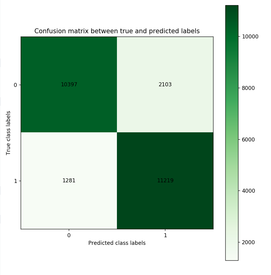
Figure 12 is the resultant confusion matrix for our sentiment analysis problem. The first row in the table represents the true 0 (or negative sentiment) class labels (we have 10,397 + 2,103 = 12,500 reviews with negative sentiment). The second row represents the true 1 (or positive sentiment) class labels (Again, we have 1,281 + 11,219 = 12,500 reviews with positive sentiment). The left column represents the predicted negative sentiment class labels (Our RNN predicted 10,397 + 1,281 = 11,678 reviews as having a negative sentiment). The right column represents the predicted positive class labels (Our RNN predicted 11,219 + 2,103 = 13,322 reviews as having a positive sentiment).Looking at the bottom right cell, we see that our RNN has correctly predicted 11,219 reviews as having a positive sentiment (True positives). Looking at the top right cell, we see that our RNN has incorrectly predicted 2,103 reviews as having a positive (False positives). Similarly, looking at the top left cell, we see that our RNN has correctly predicted 10,397 reviews as having negative sentiment (True negative). Finally, looking at the bottom left cell, we see that our RNN has incorrectly predicted 1,281 reviews as negative (False negative). Given these numbers we can calculate Precision, Recall, and the F score as follows:
\[Precision = \frac{\text{True positives}}{\text{True positives + False positives}} = \frac{11,219}{11,219 + 2,102} = 0.84\] \[Recall = \frac{\text{True positives}}{\text{True positives + False negatives}} = \frac{11,219}{11,219 + 1,281} = 0.89\] \[F score = \frac{2 * \text{Precision * Recall}}{\text{Precision + Recall}} = \frac{2 * 0.84 * 0.89}{0.84 + 0.89} = 0.86\]Conclusion
In this tutorial, we briefly reviewed feedforward neural networks, explained how recurrent neural networks are different, and discussed various RNN input/output and architectures. We also discussed various text representation and preprocessing schemes and used Galaxy to solve a sentiment classification problem using RNN on IMDB movie reviews dataset.
Frequently Asked Questions
Have questions about this tutorial? Check out the tutorial FAQ page or the FAQ page for the Statistics and machine learning topic to see if your question is listed there. If not, please ask your question on the GTN Gitter Channel or the Galaxy Help ForumReferences
- Newell, A., 1969 Perceptrons. An Introduction to Computational Geometry. Marvin Minsky and Seymour Papert. M.I.T. Press, Cambridge, Mass., 1969. vi + 258 pp., illus. Cloth, 12; paper, 4.95. Science 165: 780–782. 10.1126/science.165.3895.780 https://science.sciencemag.org/content/165/3895/780
- Rumelhart, D. E., G. E. Hinton, and R. J. Williams, 1986 Learning representations by back-propagating errors. Nature 323: 533–536. 10.1038/323533a0
- Cybenko, G., 1989 Approximation by superpositions of a sigmoidal function. Mathematics of Control, Signals and Systems 2: 303–314. 10.1007/BF02551274
- Hochreiter, S., and J. Schmidhuber, 1997 Long short-term memory. Neural computation 9: 1735–1780.
- Maas, A. L., R. E. Daly, P. T. Pham, D. Huang, A. Y. Ng et al., 2011 Learning Word Vectors for Sentiment Analysis. Proceedings of the 49th Annual Meeting of the Association for Computational Linguistics: Human Language Technologies 142–150. http://www.aclweb.org/anthology/P11-1015
- Cho, K., B. van Merriënboer, C. Gulcehre, D. Bahdanau, F. Bougares et al., 2014 Learning Phrase Representations using RNN Encoder–Decoder for Statistical Machine Translation. Proceedings of the 2014 Conference on Empirical Methods in Natural Language Processing (EMNLP) 1724–1734. 10.3115/v1/D14-1179 https://www.aclweb.org/anthology/D14-1179
- Wen, T.-H., M. Gasic, N. Mrksic, P.-hao Su, D. Vandyke et al., 2015 Semantically Conditioned LSTM-based Natural Language Generation for Spoken Dialogue Systems. Proceedings of the 2015 Conference on Empirical Methods in Natural Language Processing 1711–1721. 10.18653/v1/D15-1199 https://www.aclweb.org/anthology/D15-1199
- Lim, W., D. Jang, and T. Lee, 2016 Speech emotion recognition using convolutional and Recurrent Neural Networks. 2016 Asia-Pacific Signal and Information Processing Association Annual Summit and Conference (APSIPA) 1–4. 10.1109/APSIPA.2016.7820699
- Karpathy, A., and L. Fei-Fei, 2017 Deep Visual-Semantic Alignments for Generating Image Descriptions. IEEE Transactions on Pattern Analysis and Machine Intelligence 39: 664–676. 10.1109/TPAMI.2016.2598339
- Li, P., W. Lam, L. Bing, and Z. Wang, 2017 Deep Recurrent Generative Decoder for Abstractive Text Summarization. Proceedings of the 2017 Conference on Empirical Methods in Natural Language Processing 2091–2100. 10.18653/v1/D17-1222 https://www.aclweb.org/anthology/D17-1222
- Nwankpa, C., W. Ijomah, A. Gachagan, and S. Marshall, 2018 Activation Functions: Comparison of trends in Practice and Research for Deep Learning. CoRR abs/1811.03378: http://arxiv.org/abs/1811.03378
- Tatbul, N., T. J. Lee, S. Zdonik, M. Alam, and J. Gottschlich, 2018 Precision and Recall for Time Series. Advances in Neural Information Processing Systems 31: 1920–1930. https://proceedings.neurips.cc/paper/2018/file/8f468c873a32bb0619eaeb2050ba45d1-Paper.pdf
Feedback
Did you use this material as an instructor? Feel free to give us feedback on how it went.
Did you use this material as a learner or student? Click the form below to leave feedback.
Citing this Tutorial
- Kaivan Kamali, 2021 Deep Learning (Part 2) - Recurrent neural networks (RNN) (Galaxy Training Materials). https://training.galaxyproject.org/training-material/topics/statistics/tutorials/RNN/tutorial.html Online; accessed TODAY
- Batut et al., 2018 Community-Driven Data Analysis Training for Biology Cell Systems 10.1016/j.cels.2018.05.012
details BibTeX
@misc{statistics-RNN,
author = "Kaivan Kamali",
title = "Deep Learning (Part 2) - Recurrent neural networks (RNN) (Galaxy Training Materials)",
year = "2021",
month = "05",
day = "21"
url = "\url{https://training.galaxyproject.org/training-material/topics/statistics/tutorials/RNN/tutorial.html}",
note = "[Online; accessed TODAY]"
}
@article{Batut_2018,
    doi = {10.1016/j.cels.2018.05.012},
    url = {https://doi.org/10.1016%2Fj.cels.2018.05.012},
    year = 2018,
    month = {jun},
    publisher = {Elsevier {BV}},
    volume = {6},
    number = {6},
    pages = {752--758.e1},
    author = {B{\'{e}}r{\'{e}}nice Batut and Saskia Hiltemann and Andrea Bagnacani and Dannon Baker and Vivek Bhardwaj and Clemens Blank and Anthony Bretaudeau and Loraine Brillet-Gu{\'{e}}guen and Martin {\v{C}}ech and John Chilton and Dave Clements and Olivia Doppelt-Azeroual and Anika Erxleben and Mallory Ann Freeberg and Simon Gladman and Youri Hoogstrate and Hans-Rudolf Hotz and Torsten Houwaart and Pratik Jagtap and Delphine Larivi{\`{e}}re and Gildas Le Corguill{\'{e}} and Thomas Manke and Fabien Mareuil and Fidel Ram{\'{\i}}rez and Devon Ryan and Florian Christoph Sigloch and Nicola Soranzo and Joachim Wolff and Pavankumar Videm and Markus Wolfien and Aisanjiang Wubuli and Dilmurat Yusuf and James Taylor and Rolf Backofen and Anton Nekrutenko and Björn Grüning},
    title = {Community-Driven Data Analysis Training for Biology},
    journal = {Cell Systems}
}
Congratulations on successfully completing this tutorial!
Do you want to extend your knowledge? Follow one of our recommended follow-up trainings:
- Statistics and machine learning
- Deep Learning (Part 3) - Convolutional neural networks (CNN): slides slides - tutorial hands-on
 Questions:
